Visualizing Digital Elevation Maps
What is the highest geographic point in your country? The lowest? What if you could answer both questions at a glance?
In this tutorial we’ll demonstrate how to convert a Digital Elevation Model (DEM) into a visualization suitable for use in a website or other application. A DEM is simply a 3D representation of a terrain’s surface. Typically these are used for mapping the Earth’s surface, but the same principle applies to mapping the Moon, other planets, or even microscopic surfaces. You may have encountered a similar concept in computer graphics, where it’s referred to as a heightmap.
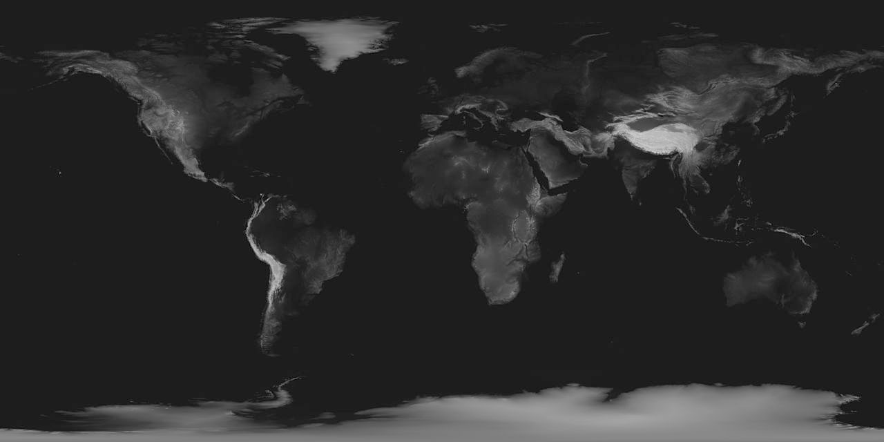
Here’s what a DEM of the earth looks like (white regions represent higher elevation). Note the prominence of the Rockies, Andes, and Himalayan mountain ranges:
DEMs have many applications:
- Estimating potential sites for avalanches or landslides
- Modeling water flow for hydrology
- Digital flight planning
- Improving satellite navigation, such as GPS
- Optimizing position of RF sources (e.g. cell towers)
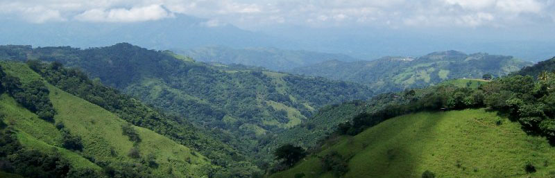
For this example we’ll use a DEM to create a topographic map of Costa Rica. Costa Rica is an especially interesting example as it contains a variety of surface features ranging from relatively flat plains to rugged peaks.
To begin, we’ll need to collect raw topographical data. Fortunately, NASA has taken care of this for us with the Shuttle Radar Topography Mission (SRTM), a research effort that collected global elevation data with a resolution of 30 m per pixel.
1. Create a heightmap
The first step is to download the data, which comes in the form of “tiles” of approximately 300,000 km2. This data can be downloaded directly from the SRTM website or, more interactively, with the SRTM Tile Grabber. A complete map of Costa Rica spans four tiles:


To combine them with the correct cartographic projection we’ll use the gdalwarp function, part of the Geospatial Data Abstraction Library, an open-source package for manipulating geospatial data formats.
gdalwarp
  -r lanczos
  -te -250000 -156250 250000 156250
  -t_srs "+proj=aea +lat_1=8 +lat_2=11.5 +lat_0=9.7 +lon_0=-84.2 +x_0=0 +y_0=0"
  -ts 960 0
  srtm_19_10.tif srtm_20_10.tif srtm_19_11.tif srtm_20_11.tif
  heightmap.tiff
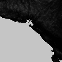
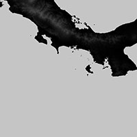
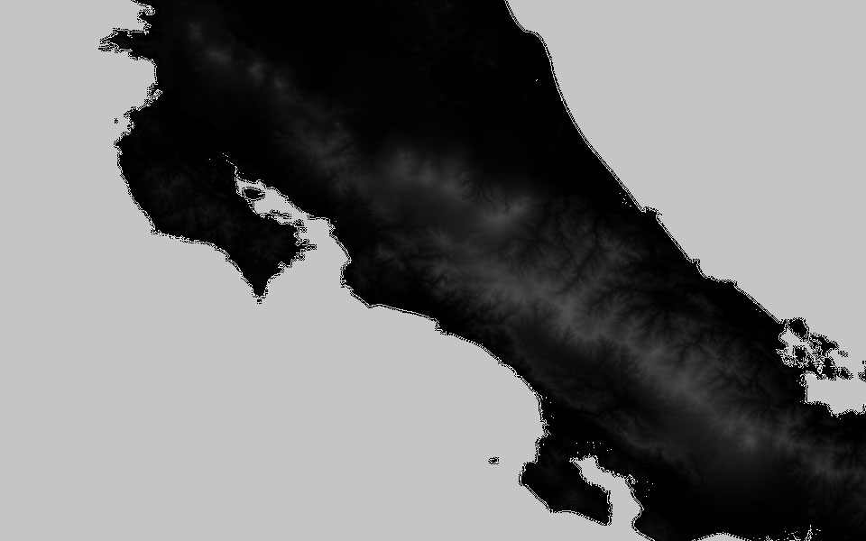
The t_srs option sets an albers equal area projection that will center on Costa Rica. The te option defines the extent of the map, using Spatial Reference System (SRS) coordinates. Lastly, the ts option specifies the output image size in pixels. Here’s what the merged and projected heightmap looks like:
2. Create color relief map
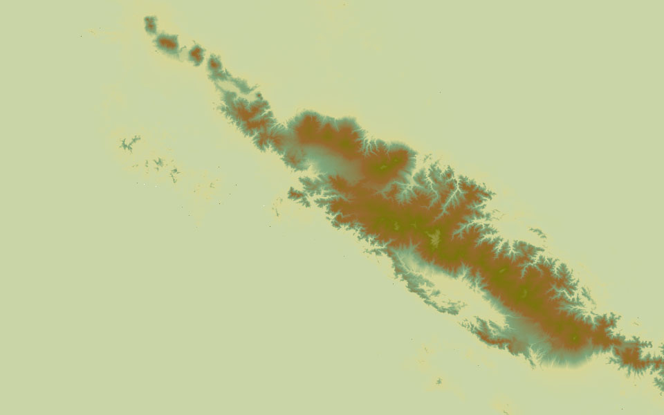
Next let’s add some color. We’ll do this with the GDAL utility gdaldem which will combine the heightmap we generated with a list of colors. The colors are defined as a list of [elevation x y z] tuples, which gdaldem will interpolate. We’ll choose green for low elevation and brown for high elevation, but the choice of colors is arbitrary.
gdaldem
  color-relief
  heightmap.tiff
  color_relief.txt
  hill-relief-c.tiff
Where color_relief.txt contains the following values:
| Elevation (m) | RRed | GGreen | BBlue | |
| 65535 | 255 | 255 | 255 | |
| 5800 | 254 | 254 | 254 | |
| 3000 | 121 | 117 | 10 | |
| 1500 | 151 | 106 | 47 | |
| 800 | 127 | 166 | 122 | |
| 500 | 213 | 213 | 149 | |
| 1 | 201 | 213 | 166 |
3. Create a shaded relief map
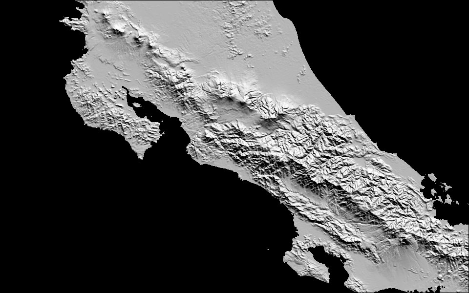
To add a bit more visual interest we can create a shaded relief map that simulates the appearance of light coming from an angle simulating light coming from an angle. We turn again to the gdaldem utility, this time with the hillshade option.
gdaldem
  hillshade
  relief.tiff
  hill-relief-shaded.tiff
  -z 4 -az 20
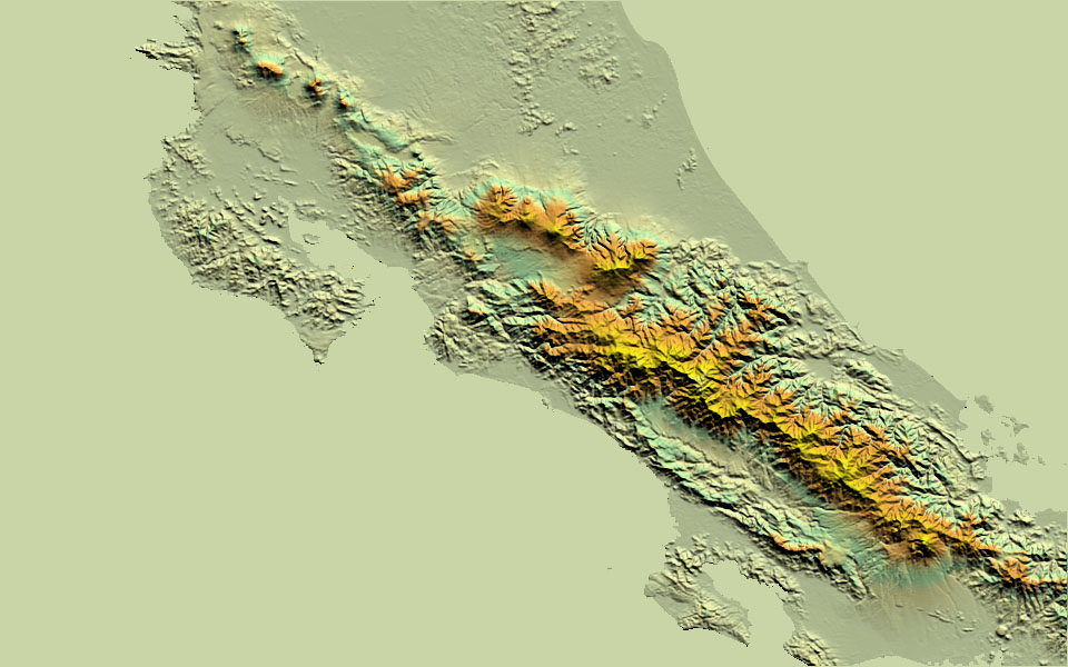
4. Merge shade and color
Next we’ll combine the color and shaded relief maps with a simple python script (see the end of this tutorial for the code):
hsv_merge.py
  hill-relief-c.tiff
  hill-relief-shaded.tiff
  hill-relief-merged.tiff
5. Add costa rica geographic data
Looking pretty good! As a last step let’s incorporate geographic data so we can clearly see the country’s boundaries. To do this, we’ll use get Costa Rica’s administrative boundaries from GADM.org, and convert them into a format suitable for use on the web, namely TopoJSON.
For reasons that aren’t terribly interesting we’ll have to first convert from GDAL’s shapefile format to GeoJSON and then to TopoJSON using GDAL’s ogr2ogr and Mike Bostock’s topojson utilities, respectively:
curl -o CRI_adm.zip http://gadm.org/data/shp/CRI_adm.zip
ogr2ogr -f GeoJSON costarica.json CRI_adm0.shp
topojson -p name=NAME -p name -q 1e4 -o costarica_min_topo.json costarica.json
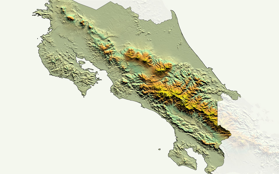
End result
With a a little D3js magic (i.e., “left as an exercise for the reader”) we can combine the geographic data with the merged relief map. Feel free to send me an email with any questions or comments.
BONUS: Simulating RF Propagation
Now that we have our DEM, what do we do with it? One application where knowledge of terrain is important is in radiofrequency (RF) propagation.
Suppose you’re a cell phone provider and you want to bring service to a new region. One of the most significant costs is the installation of cell towers. Too many towers gets expensive, but too few towers may result in spotty or unreliable service. How many towers do you put up, and where?
Recall that cell phone signals are heavily attenuated by terrain. We can imagine a simple radio propagation model where the signal is attenuated by some constant factor per meter of terrain traversed. Thus a tower located on a mountain top would have a broad coverage area relative to a tower placed in a valley.
In the simulation below, try clicking on various points on the map to place virtual cell phone towers. Notice how the signal is affected by surrounding terrain features. Can you think of a way to optimize tower placement to minimize their numbers?
Want to learn more? Join our meetup group! Bethesda Data Science Meetup